
39 Javanotes 9.0, Section 9.1 — Recursion
Section 9.1
Recursion
At one time or another, you’ve probably been told
that you can’t define something in terms of itself. Nevertheless, if it’s done
right, defining something at least partially in terms of itself can be a very
powerful technique. A recursive definition is one
that uses the concept or thing that is being defined as part of the definition.
For example: An “ancestor” is either a parent or an ancestor of a parent. A
“sentence” can be, among other things, two sentences joined by a conjunction
such as “and.” A “directory” is a part of a disk drive that can hold files and
directories. In mathematics, a “set” is a collection of elements, which can themselves be
sets. A “statement” in Java can be a while statement, which is
made up of the word “while”, a boolean-valued condition, and a statement.
Recursive definitions can describe very complex situations with just a few
words. A definition of the term “ancestor” without using recursion might go
something like “a parent, or a grandparent, or a great-grandparent, or a
great-great-grandparent, and so on.” But saying “and so on” is not very
rigorous. (I’ve often thought that recursion is really just a rigorous way of
saying “and so on.”) You run into the same problem if you try to define a
“directory” as “a file that is a list of files, where some of the files can be
lists of files, where some of those files can be lists of files, and so
on.” Trying to describe what a Java statement can look like, without using
recursion in the definition, would be difficult and probably pretty comical.
Recursion can be used as a programming technique. A
recursive subroutine (or recursive method)
is one that calls itself, either directly
or indirectly. To say that a subroutine calls itself directly means that its
definition contains a subroutine call statement that calls the subroutine that
is being defined. To say that a subroutine calls itself indirectly means that
it calls a second subroutine which in turn calls the first subroutine (either
directly or indirectly). A recursive subroutine can define a complex task in
just a few lines of code. In the rest of this section, we’ll look at a variety
of examples, and we’ll see other examples in the rest of the book.
9.1.1 Recursive Binary Search
Let’s start with an example that you’ve seen before: the binary search
algorithm from Subsection 7.5.1. Binary search is used
to find a specified value in a sorted list of items (or, if it does not occur
in the list, to determine that fact). The idea is to test the element in the
middle of the list. If that element is equal to the specified value, you are
done. If the specified value is less than the middle element of the list, then
you should search for the value in the first half of the list. Otherwise, you
should search for the value in the second half of the list. The method used to
search for the value in the first or second half of the list is binary search.
That is, you look at the middle element in the half of the list that is still
under consideration, and either you’ve found the value you are looking for, or
you have to apply binary search to one half of the remaining elements. And so
on! This is a recursive description, and we can write a recursive subroutine to
implement it.
Before we can do that, though, there are two considerations that we need to
take into account. Each of these illustrates an important general fact about
recursive subroutines. First of all, the binary search algorithm begins by
looking at the “middle element of the list.” But what if the list is empty? If
there are no elements in the list, then it is impossible to look at the middle
element. In the terminology of Subsection 8.2.2, having
a non-empty list is a “precondition” for looking at the middle element, and
this is a clue that we have to modify the algorithm to take this precondition
into account. What should we do if we find ourselves searching for a specified
value in an empty list? The answer is easy: If the list is empty, we can be sure that the
value does not occur in the list, so we can give the answer without any further work.
An empty list is a base case
for the binary search algorithm. A base case for a recursive
algorithm is a case that is handled directly, rather than by applying the
algorithm recursively. The binary search algorithm actually has another type of
base case: If we find the element we are looking for in the middle of the list,
we are done. There is no need for further recursion.
The second consideration has to do with the parameters to the subroutine.
The problem is phrased in terms of searching for a value in a list. In the
original, non-recursive binary search subroutine, the list was given as an
array. However, in the recursive approach, we have to be able to apply the
subroutine recursively to just a part of the original list. Where the
original subroutine was designed to search an entire array, the recursive
subroutine must be able to search part of an array. The parameters to the
subroutine must tell it what part of the array to search. This illustrates a
general fact that in order to solve a problem recursively, it is often
necessary to generalize the problem slightly.
Here is a recursive binary search algorithm that searches for a given value
in part of an array of integers:
/**
 * Search in the array A in positions numbered loIndex to hiIndex,
 * inclusive, for the specified value.  If the value is found, return
 * the index in the array where it occurs.  If the value is not found,
 * return -1.  Precondition:  The array must be sorted into increasing
 * order.
 */
static int binarySearch(int[] A, int loIndex, int hiIndex, int value) {

   if (loIndex > hiIndex) {
         // The starting position comes after the final index,
         // so there are actually no elements in the specified
         // range.  The value does not occur in this empty list!
      return -1;
   }

   else {
         // Look at the middle position in the list.  If the
         // value occurs at that position, return that position.
         // Otherwise, search recursively in either the first
         // half or the second half of the list.
      int middle = (loIndex + hiIndex) / 2;
      if (value == A[middle])
         return middle;
      else if (value < A[middle])
         return binarySearch(A, loIndex, middle - 1, value);
      else   // value must be > A[middle]
         return binarySearch(A, middle + 1, hiIndex, value);
   }

} // end binarySearch()
In this routine, the parameters loIndex and hiIndex
specify the part of the array that is to be searched. To search an entire
array, it is only necessary to call binarySearch(A, 0, A.length – 1,
value). In the two base cases—when there are no elements in the
specified range of indices and when the value is found in the middle of the
range—the subroutine can return an answer immediately, without using
recursion. In the other cases, it uses a recursive call to compute the answer
and returns that answer.
Most people find it difficult at first to convince themselves that recursion
actually works. The key is to note two things that must be true for recursion
to work properly: There must be one or more base cases, which can be handled
without using recursion. And when recursion is applied during the solution of a
problem, it must be applied to a problem that is in some sense smaller—that
is, closer to the base cases—than the original problem. The idea is that if
you can solve small problems and if you can reduce big problems to smaller
problems, then you can solve problems of any size. Ultimately, of course, the
big problems have to be reduced, possibly in many, many steps, to the very
smallest problems (the base cases). Doing so might involve an immense amount of
detailed bookkeeping. But the computer does that bookkeeping, not you! As a
programmer, you lay out the big picture: the base cases and the reduction of
big problems to smaller problems. The computer takes care of the details
involved in reducing a big problem, in many steps, all the way down to base
cases. Trying to think through this reduction in detail is likely to drive you
crazy, and will probably make you think that recursion is hard. Whereas in
fact, recursion is an elegant and powerful method that is often the simplest
approach to solving a complex problem.
A common error in writing recursive subroutines is to violate one of the two
rules: There must be one or more base cases, and when the subroutine is applied
recursively, it must be applied to a problem that is smaller than the original
problem. If these rules are violated, the result can be an
infinite recursion, where the subroutine keeps calling itself
over and over, without ever reaching a base case. Infinite recursion is similar
to an infinite loop. However, since each recursive call to the subroutine uses
up some of the computer’s memory, a program that is stuck in an infinite
recursion will run out of memory and crash before long. In Java, the program
will crash with an exception of type StackOverflowError.
9.1.2 Towers of Hanoi
We have been studying an algorithm, binary search, that
can easily be implemented with a while loop, instead of with
recursion. Next, we
turn to a problem that is easy to solve with recursion but difficult to solve
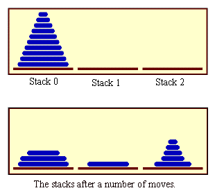
without it. This is a standard example known as “The Towers of Hanoi.” The
problem involves a stack of various-sized disks, piled up on a base in order of
decreasing size. The object is to move the stack from one base to another,
subject to two rules: Only one disk can be moved at a time, and no disk can
ever be placed on top of a smaller disk. There is a third base that can be used
as a “spare.” The starting situation for a stack of ten disks is shown in the top half
of the following picture. The situation after a number of moves have been made
is shown in the bottom half of the picture. (These illustrations are from a sample
program from Chapter 12,
TowersOfHanoiGUI.java, which displays an
animation of the step-by-step solution of the problem; however, that
program uses some techniques that you haven’t learned yet.)
The problem is to move ten disks from Stack 0 to Stack 1, subject to the rules
given above. Stack 2 can be used as a spare location. Can we reduce this to smaller
problems of the same type, possibly generalizing the problem a bit to make this
possible? It seems natural to consider the size of the problem to be the number
of disks to be moved. If there are N disks in Stack 0, we know that we
will eventually have to move the bottom disk from Stack 0 to Stack 1. But
before we can do that, according to the rules, the first N-1 disks
must be on Stack 2. Once we’ve moved the N-th disk to Stack 1, we must
move the other N-1 disks from Stack 2 to Stack 1 to complete the
solution. But moving N-1 disks is the same type of problem as moving
N disks, except that it’s a smaller version of the problem. This is
exactly what we need to do recursion! The problem has to be generalized a bit,
because the smaller problems involve moving disks from Stack 0 to Stack 2 or
from Stack 2 to Stack 1, instead of from Stack 0 to Stack 1. In the recursive
subroutine that solves the problem, the stacks that serve as the source and
destination of the disks have to be specified. It’s also convenient to specify
the stack that is to be used as a spare, even though we could figure that out
from the other two parameters. The base case is when there is only one disk to
be moved. The solution in this case is trivial: Just move the disk in one step.
Here is a version of the subroutine that will print out step-by-step
instructions for solving the problem:
/**
 * Solve the problem of moving the number of disks specified
 * by the first parameter from the stack specified by the
 * second parameter to the stack specified by the third
 * parameter.  The stack specified by the fourth parameter
 * is available for use as a spare.  Stacks are specified by
 * number: 0, 1, or 2.
 */
static void towersOfHanoi(int disks, int from, int to, int spare) {
    if (disks == 1) {
            // There is only one disk to be moved.  Just move it.
        System.out.printf("Move disk 1 from stack %d to stack %d%n",
                               from, to);
    }
    else {
            // Move all but one disk to the spare stack, then
            // move the bottom disk, then put all the other
            // disks on top of it.
        towersOfHanoi(disks-1, from, spare, to);
        System.out.printf("Move disk %d from stack %d to stack %d%n",
                              disks, from, to);
        towersOfHanoi(disks-1, spare, to, from);
    }
}
This subroutine just expresses the natural recursive solution. The recursion
works because each recursive call involves a smaller number of disks, and the
problem is trivial to solve in the base case, when there is only one disk. To
solve the “top level” problem of moving N disks from Stack 0 to Stack
1, the subroutine should be called with the command TowersOfHanoi(N,0,1,2). The
subroutine is used in the sample program TowersOfHanoi.java.
Here, for example, is the output from the program when it is run
with the number of disks set equal to 4:
Move disk 1 from stack 0 to stack 2
Move disk 2 from stack 0 to stack 1
Move disk 1 from stack 2 to stack 1
Move disk 3 from stack 0 to stack 2
Move disk 1 from stack 1 to stack 0
Move disk 2 from stack 1 to stack 2
Move disk 1 from stack 0 to stack 2
Move disk 4 from stack 0 to stack 1
Move disk 1 from stack 2 to stack 1
Move disk 2 from stack 2 to stack 0
Move disk 1 from stack 1 to stack 0
Move disk 3 from stack 2 to stack 1
Move disk 1 from stack 0 to stack 2
Move disk 2 from stack 0 to stack 1
Move disk 1 from stack 2 to stack 1
The output of this program shows you a mass of detail that you don’t really want to
think about! The difficulty of following the details contrasts sharply with the
simplicity and elegance of the recursive solution. Of course, you really want
to leave the details to the computer.
(You might think about what happens when the
precondition that the number of disks is positive is violated. The result is
an example of infinite recursion.)
There is, by the way, a story that explains the name of this problem.
According to this story, on the first day of creation, a group of monks in an
isolated tower near Hanoi were given a stack of 64 disks and were assigned the
task of moving one disk every day, according to the rules of the Towers of
Hanoi problem. On the day that they complete their task of moving all the disks
from one stack to another, the universe will come to an end. But don’t worry.
The number of steps required to solve the problem for N disks is
2N – 1, and 264 – 1 days is over 50,000,000,000,000
years. We have a long way to go.
(In the terminology of Section 8.5, the Towers of Hanoi
algorithm has a run time that is Θ(2n), where n is the number
of disks that have to be moved.
Since the exponential function 2n grows
so quickly, the Towers of Hanoi problem can be solved in practice only for a small
number of disks.)
By the way, in addition to the graphical Towers of Hanoi program, mentioned above,
there are two more demo programs that you might want to look at. Each program
provides a visual demonstration of a recursive algorithm. In
Maze.java, recursion is used to solve a maze.
In LittlePentominos.java, it is used to solve
a well-known kind of puzzle. (LittlePentominos.java also requires
the file MosaicCanvas.java.) It would be useful
to run the programs and watch them for a while, but the source code
uses some techniques that won’t be covered until Chapter 12.
The Maze program first creates a random maze. It then tries to solve the maze
by finding a path through the maze from the upper left corner to the lower
right corner. This problem is actually very similar to a “blob-counting”
problem that is considered later in this section.
The recursive maze-solving routine starts from a given square, and it
visits each neighboring square and calls itself recursively from there. The
recursion ends if the routine finds itself at the lower right corner of the
maze. When it can’t find a solution from a square, it “backs up” out of
that square and tries somewhere else. This common technique is referred to as
recursive backtracking.
The LittlePentominos program is an implementation of a classic puzzle. A pentomino
is a connected figure made up of five equal-sized squares. There are exactly
twelve figures that can be made in this way, not counting all the possible
rotations and reflections of the basic figures. The problem is to place the
twelve pentominos on an 8-by-8 board in which four of the squares have already
been marked as filled. The recursive solution looks at a board that has already
been partially filled with pentominos. The subroutine looks at each remaining
piece in turn. It tries to place that piece in the next available place on the
board. If the piece fits, it calls itself recursively to try to fill in the
rest of the solution. If that fails, then the subroutine goes on to the next
piece—another example of recursive backtracking.
A generalized version of the pentominos program with many more features
can be found at
https://math.hws.edu/eck/js/pentominos/pentominos.html.
9.1.3 A Recursive Sorting Algorithm
Turning next to an application that is perhaps more practical, we’ll look at
a recursive algorithm for sorting an array. The selection sort and insertion
sort algorithms, which were covered in Section 7.5,
are fairly simple, but they are rather slow
when applied to large arrays. Faster sorting algorithms are available. One of
these is Quicksort, a recursive algorithm which turns out to be the fastest
sorting algorithm in most situations.
The Quicksort algorithm is based on a simple but clever idea: Given a list
of items, select any item from the list. This item is called the
pivot. (In practice, I’ll just use the first item in the
list.) Move all the items that are smaller than the pivot to the beginning of
the list, and move all the items that are larger than the pivot to the end of
the list. Now, put the pivot between the two groups of items. This puts the
pivot in the position that it will occupy in the final, completely sorted
array. It will not have to be moved again. We’ll refer to this procedure as
QuicksortStep.

QuicksortStep is not recursive. It is used as a subroutine by Quicksort. The
speed of Quicksort depends on having a fast implementation of QuicksortStep.
Since it’s not the main point of this discussion, I present one without much
comment.
/**
 * Apply QuicksortStep to the list of items in locations lo through hi
 * in the array A.  The value returned by this routine is the final
 * position of the pivot item in the array.
 */
 static int quicksortStep(int[] A, int lo, int hi) {

    int pivot = A[lo];  // Get the pivot value.

    // The numbers hi and lo mark the endpoints of a range
    // of numbers that have not yet been tested.  Decrease hi
    // and increase lo until they become equal, moving numbers
    // bigger than pivot so that they lie above hi and moving
    // numbers less than the pivot so that they lie below lo.
    // When we begin, A[lo] is an available space, since its
    // value has been moved into the local variable, pivot.

    while (hi > lo) {

       // Loop invariant (See Subsection Subsection 8.2.3):  A[i] <= pivot
       // for i < lo, and A[i] >= pivot for i > hi.

       while (hi > lo && A[hi] >= pivot) {
             // Move hi down past numbers greater than pivot.
             // These numbers do not have to be moved.
          hi--;
       }

       if (hi == lo)
          break;

       // The number A[hi] is less than pivot.  Move it into
       // the available space at A[lo], leaving an available
       // space at A[hi].

       A[lo] = A[hi];
       lo++;

       while (hi > lo && A[lo] <= pivot) {
             // Move lo up past numbers less than pivot.
             // These numbers do not have to be moved.
          lo++;
       }

       if (hi == lo)
          break;

       // The number A[lo] is greater than pivot.  Move it into
       // the available space at A[hi], leaving an available
       // space at A[lo].

       A[hi] = A[lo];
       hi--;

    } // end while

    // At this point, lo has become equal to hi, and there is
    // an available space at that position.  This position lies
    // between numbers less than pivot and numbers greater than
    // pivot.  Put pivot in this space and return its location.

    A[lo] = pivot;
    return lo;

 }  // end QuicksortStep
With this subroutine in hand, Quicksort is easy. The Quicksort algorithm for
sorting a list consists of applying QuicksortStep to the list, then applying
Quicksort recursively to the items that lie to the left of the new position of the
pivot and to the
items that lie to the right of that position. Of course, we need base cases. If the
list has only one item, or no items, then the list is already as sorted as it
can ever be, so Quicksort doesn’t have to do anything in these cases.
/**
 * Apply quicksort to put the array elements between
 * position lo and position hi into increasing order.
 */
static void quicksort(int[] A, int lo, int hi) {
   if (hi <= lo) {
         // The list has length one or zero.  Nothing needs
         // to be done, so just return from the subroutine.
      return;
   }
   else {
         // Apply quicksortStep and get the new pivot position.
         // Then apply quicksort to sort the items that
         // precede the pivot and the items that follow it.
      int pivotPosition = quicksortStep(A, lo, hi);
      quicksort(A, lo, pivotPosition - 1);
      quicksort(A, pivotPosition + 1, hi);
   }
}
As usual, we had to generalize the problem. The original problem was to sort
an array, but the recursive algorithm is set up to sort a specified part of an
array. To sort an entire array, A, using the quickSort()
subroutine, you would call quicksort(A, 0, A.length – 1).
Quicksort is an interesting example from the point of view of the analysis
of algorithms (Section 8.5), because its average case
run time differs greatly from its worst case run time. Here is a very informal
analysis, starting with the average case: Note that an application of
quicksortStep divides a problem into two sub-problems. On
the average, the subproblems will be of approximately the same size. A
problem of size n is divided into two problems that are roughly of size
n/2; these are then divided into four problems that are roughly of size
n/4; and so on. Since the problem size is divided by 2 on each level,
there will be approximately log(n) levels of subdivision.
The amount of processing on each level is proportional to n. (On the
top level, each element in the array is looked at and possibly moved.
On the second level, where there are two subproblems, every element but
one in the array is part of one of those two subproblems and must be
looked at and possibly moved, so there is a total of about n steps
in both subproblems combined. Similarly, on
the third level, there are four subproblems and a total of
about n steps in the four subproblems on that level….)
With a total of n steps on each level and approximately log(n) levels
in the average case, the average case run time for Quicksort is
Θ(n*log(n)). This analysis assumes that quicksortStep divides
a problem into two approximately equal parts. However, in the worst case,
each application of quicksortStep divides a problem of size n into
a problem of size 0 and a problem of size n-1. This happens when the
pivot element ends up at the beginning or end of the array. In this
worst case, there are n levels of subproblems, and the worst-case run
time is Θ(n2). The worst case is very rare—it
depends on the items in the array being arranged in a very special way,
so the average performance of Quicksort can be very good even though
it is not so good in certain rare cases. (One of these “rare” cases is
when the original array is already sorted or almost sorted, which is
really not all that rare in practice. Applying the Quicksort
algorithm as given above to a large sorted array will take a long time.
One way to avoid that—with high probablility—is to pick the pivot for QuickSort step at random,
rather than always using the first item.)
There are sorting algorithms that have both an average case and a worst case
run time of Θ(n*log(n)).
One example that is fairly easy to understand is MergeSort, which you can
look up if you are interested.
9.1.4 Blob Counting
Next, we will look at counting the number of squares in a group of
connected squares. I call a group of connected squares a “blob,” and the sample program
that we will consider is Blobs.java.
The program displays a grid of small white, gray,
and red squares. Here is a screenshot from the program, showing the
grid of squares along with some controls:
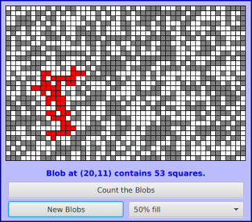
The gray or red squares are considered to be
“filled” and the white squares are “empty.” For the purposes of this example, we
define a “blob” to consist of a filled square and all the filled squares that
can be reached from it by moving up, down, left, and right through other filled
squares. If the user clicks on any filled square in the program, the computer will
count the squares in the blob that contains the clicked square, and it will change the color of
those squares to red. In the picture, one of the blobs is shown in red.
The program has several controls. There is a
“New Blobs” button; clicking this button will create a new random
pattern in the grid. A pop-up menu specifies the approximate percentage of
squares that will be filled in the new pattern. The more filled squares, the
larger the blobs. And a button labeled “Count the Blobs” will tell you how many
different blobs there are in the pattern.
Recursion is used in this program to count the number of squares in a blob.
Without recursion, this would be a very difficult thing to implement. Recursion
makes it relatively easy, but it still requires a new technique, which is also
useful in a number of other applications.
The data for the grid of squares is stored in a two dimensional array of
boolean values,
boolean[][] filled;
The value of filled[r][c] is true if the square in row r
and in column c of the grid is filled. The number of rows in the grid
is stored in an instance variable named rows, and the number of
columns is stored in columns. The program uses a recursive instance
method named getBlobSize(r,c) to count the number of squares in a blob.
The parameters r and c tell which blob to count, namely
the blob that includes the square in a row r and column c. If
there is no filled square at position (r,c), then the answer is zero.
Otherwise, getBlobSize() has to count all the filled squares that can
be reached from the square at position (r,c). The idea is to use
getBlobSize() recursively to get the number of filled squares that can
be reached from each of the neighboring positions: (r+1,c),
(r-1,c), (r,c+1), and (r,c-1). Add up these numbers,
and add one to count the square at (r,c) itself, and you get the total
number of filled squares that can be reached from (r,c). Here is an
implementation of this algorithm, as stated. Unfortunately, it has a serious
flaw: It leads to an infinite recursion!
int getBlobSize(int r, int c) {  // BUGGY, INCORRECT VERSION!!
      // This INCORRECT method tries to count all the filled
      // squares that can be reached from position (r,c) in the grid.
   if (r < 0 || r >= rows || c < 0 || c >= columns) {
         // This position is not in the grid, so there is
         // no blob at this position.  Return a blob size of zero.
      return 0;
   }
   if (filled[r][c] == false) {
        // This square is not part of a blob, so return zero.
      return 0;
   }
   int size = 1;  // Count the square at this position, then count the
                  //   the blobs that are connected to this square
                  //   horizontally or vertically.
   size += getBlobSize(r-1,c);
   size += getBlobSize(r+1,c);
   size += getBlobSize(r,c-1);
   size += getBlobSize(r,c+1);
   return size;
}  // end INCORRECT getBlobSize()
Unfortunately, this routine will count the same square more than once. In
fact, if there are at least two squares in the blob,
then it will try to count each square infinitely often! Think of yourself
standing at position (r,c) and trying to follow these instructions.
The first instruction tells you to move up one row. You do that, and then you
apply the same procedure. As one of the steps in that procedure, you have to
move down one row and apply the same procedure yet again. But that puts
you back at position (r,c)! From there, you move up one row, and from
there you move down one row…. Back and forth forever! We have to make sure
that a square is only counted and processed once, so we don’t end up going
around in circles. The solution is to leave a trail of breadcrumbs—or on the
computer a trail of boolean values—to mark the squares that you’ve
already visited. Once a square is marked as visited, it won’t be processed
again. The remaining, unvisited squares are reduced in number, so definite
progress has been made in reducing the size of the problem. Infinite recursion
is avoided!
A second boolean array, visited[r][c], is used to keep track of
which squares have already been visited and processed. It is assumed that all
the values in this array are set to false before getBlobSize() is
called. As getBlobSize() encounters unvisited squares, it marks them
as visited by setting the corresponding entry in the visited array to
true. When getBlobSize() encounters a square that it has already
visited, it doesn’t count it or process it further. The technique of “marking”
items as they are encountered is one that is used over and over in the programming
of recursive algorithms. Here is the corrected version of
getBlobSize(), with changes shown in red italic:
/**
 * Counts the squares in the blob at position (r,c) in the
 * grid.  Squares are only counted if they are filled and
 * unvisited.  If this routine is called for a position that
 * has been visited, the return value will be zero.
 */
int getBlobSize(int r, int c) {
   if (r < 0 || r >= rows || c < 0 || c >= columns) {
         // This position is not in the grid, so there is
         // no blob at this position.  Return a blob size of zero.
      return 0;
   }
   if (filled[r][c] == false || visited[r][c] == true) {
        // This square is not part of a blob, or else it has
        // already been counted, so return zero.
      return 0;
   }
   visited[r][c] = true;   // Mark the square as visited so that
                           //    we won't count it again during the
                           //    following recursive calls.
   int size = 1;  // Count the square at this position, then count the
                  //   the blobs that are connected to this square
                  //   horizontally or vertically.
   size += getBlobSize(r-1,c);
   size += getBlobSize(r+1,c);
   size += getBlobSize(r,c-1);
   size += getBlobSize(r,c+1);
   return size;
}  // end getBlobSize()
In the program, this method is used to determine the size of a blob when the
user clicks on a square. After getBlobSize() has performed its task,
all the squares in the blob are still marked as visited. The
method that draws the grid of squares shows visited squares in red, which makes the
blob visible.
The getBlobSize() method is also used for the other task that
can be done by the program: counting all the
blobs. This is done by the following method, which includes comments to explain
how it works:
/**
 * When the user clicks the "Count the Blobs" button, find the
 * number of blobs in the grid and report the number in the
 * message label.
 */
void countBlobs() {

   int count = 0; // Number of blobs.

   /* First clear out the visited array. The getBlobSize() method
      will mark every filled square that it finds by setting the
      corresponding element of the array to true.  Once a square
      has been marked as visited, it will stay marked until all the
      blobs have been counted.  This will prevent the same blob from
      being counted more than once. */

   for (int r = 0; r < rows; r++)
      for (int c = 0; c < columns; c++)
         visited[r][c] = false;

   /* For each position in the grid, call getBlobSize() to get the
      size of the blob at that position.  If the size is not zero,
      count a blob.  Note that if we come to a position that was part
      of a previously counted blob, getBlobSize() will return 0 and
      the blob will not be counted again. */

   for (int r = 0; r < rows; r++)
      for (int c = 0; c < columns; c++) {
         if (getBlobSize(r,c) > 0)
            count++;
      }

   draw();  // Redraw the entire grid of squares.
                // Note that all the filled squares will be red,
                //    since they have all now been visited.

   message.setText("The number of blobs is " + count);

} // end countBlobs()